The basis for the Box-Jenkins methodology consists of three phases:
- Identification
- Estimation
- Testing and applying the ARIMA model
This methodology is a multi-step model building strategy aimed at optimizing the ARIMA process. ForecastX™ automatically optimizes the best ARIMA model using Box-Jenkins. ForecastX enables you to perform data transformation and analyze the ACF and PACF charts for model selection. Box Jenkins is best used on extensively long Historical data sets with lower volatility.
The table below details the four phases of the Box-Jenkins.
| Phase | Description |
|
Model Identification |
In this phase, data is plotted (if needed) for performing transformation and differencing analysis. A data transformation stabilizes the variance within a set of data points. If necessary, difference the data to make it stationary. Also, in this phase, a first guess at the ARIMA model will be analyzed. |
|
Estimation and Forecasting |
In this phase, the model parameters are chosen based on the model that provides the lowest error term. The data is then forecasted. |
| Diagnostic Checking | The decision is made based on an analysis of the statistical accuracy of the model whether to re-run using a different model or continue using the ARIMA model diagnosed. |
| Forecasting | A forecast of the time series is generated using the ARIMA model. |
The two basic classes of components in Box-Jenkins are Non- seasonal (trend) and Seasonality.
When looking for trends within data, look for gradual increases in sales over time that do not repeat within the time range being forecasted. This (in combination with higher sales during certain times of the year (seasonality)), signifies an increase in sales from year to year that follows a seasonal pattern.
To use the Box Jenkins forecasting method:
- Click on
 and open the TutorialAirlineData.xls file.
Note: The TutorialAirlineData.xls file is a data example to demonstrate how the Box Jenkins method is used. For your company’s purposes, you will have your own data available. - Click in a cell containing data and open ForecastX by clicking on
 .
.
ForecastX displays with the Data Capture tab open.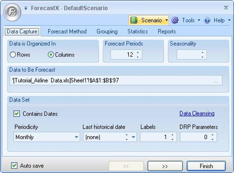
- Since your data is set up in monthly format, ensure that Contains dates is checked and monthly is selected.
- In the Forecast periods textbox, type in 36 to Forecast three years into the future.
- In the Seasonality textbox, type in 12.
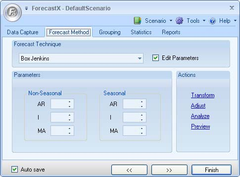
- Click the Forecast Method tab.
- In the Forecast Technique area, scroll through the list of methods and select Box Jenkins. The Box Jenkins Forecasting technique displays.
- On the Reports tab, select the Audit Trail report. The Audit Trail report includes Accuracy and Descriptive statistics.
- Click Finish.
Performing ARIMA Analysis
ForecastX includes several tools to analyze your data and assist on ARIMA selection. The following table details the tools used.
| Tools | Description |
|
Customize ARIMA Model Input |
The ability to input a non-seasonal and seasonal ARIMA model is available in ForecastX. From the Forecast Method screen, you can select Box- Jenkins and enter your own ARIMA model. |
|
Data Transformation |
This tool charts the variance and provides the functionality to transform your data. By examining the variance chart, the sophisticated forecaster can perform a log, square, and square root transformation. On the Forecast Method tab, click the Transform button and look at your variance chart. The goal is to have your data distributed evenly around the mean. |
| Data Analysis |
This chart includes the ACF and PACF chart and provides functionality to differentiate your data. The ACF and PACF (auto-correlation function and partial auto-correlation function) are used in determining whether your data is stationary. It also allows you to see seasonality and trend. As discussed previously, your data may contain both factors, and therefore must be differenced before we can choose our ARIMA model. ForecastX allows you to put in the differencing parameters and view the changes in the correlogram as you make them. |
| Differencing | On the Forecast Method tab, click the Analyze link. It is here that you can set the differencing parameters. Differencing allows you to remove the trend by subtracting adjacent data points. The correlogram displays the ACF and PACF, which show you the auto-correlations and relationships that each variable has with the past. If correlation is high, it means that the variable is predictable. |
To perform the ARIMA analysis:
- On the Forecast Method tab, scroll through the list of Forecasting techniques and select Box Jenkins.
- Check the Edit parameters checkbox and type in 1 for the Non- seasonal difference and 2 for the Seasonal difference. As you can see, only one or two correlations fall outside of the upper and lower limits.
- On the Statistics tab, select a statistic to ForecastX displays the default statistic if none are selected.
- On the Reports tab, choose the Audit Trail report.
- On the Audit tab, select the Out of Sample option to display a fitted values table.
- Click Finish.